Learning classifier systems (LCS) and Genetics-Based Machine Learning (GBML) have been using the multiplexer problem as a toy problem because of its properties; among others, its dynamic dependencies based on the input values and the exponential nature of the required solution as a function of the number of inputs. There is a great introduction why the multiplexer is interesting for LCS and GBML systems at Wilson’s XCS field-defining paper.
A simple definition [1] of the multiplexer is as follows:
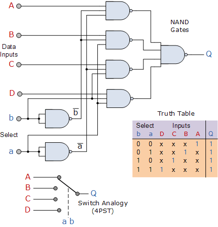
Multiplexing is the generic term used to describe the operation of sending one or more analogue or digital signals over a common transmission line at different times or speeds and as such, the device we use to do just that is called a Multiplexer.
A simple graphical representation of the 6 input (2 addresses + 4 lines) multiplexer as provided in [1] is shown below.
Let’s try to learn the solution by evolving it using Genetic Programming [2] as originally presented by John Koza.
Choosing a framework
To solve the problem we are not going to implement Koza’s initial genetic programming code from scratch. Instead we are going to do it by using DEAP [3], evolutionary computation framework for rapid prototyping and testing of ideas. DEAP is written in Python and you can just us it in a Jupiter notebook [4].
Problem definition
Imagine you have the problem defined in a CSV file. Each row is a possible input combination to the problem illustrated above. A0 and A1 represent the two address lines on the 6 input multiplexer. I0, I1, I2 and A3 the selectable lines based on the values of the address lines. Finally, O is the expected output.
| A0 | A1 | I0 | I1 | I2 | I3 | O |
|---|---|---|---|---|---|---|
| 0 | 0 | 0 | 0 | 0 | 0 | 0 |
| 0 | 0 | 0 | 0 | 0 | 1 | 0 |
| 0 | 0 | 0 | 0 | 1 | 0 | 0 |
| 0 | 0 | 0 | 0 | 1 | 1 | 0 |
| 0 | 0 | 0 | 1 | 0 | 0 | 0 |
| 0 | 0 | 0 | 1 | 0 | 1 | 0 |
| 0 | 0 | 0 | 1 | 1 | 0 | 0 |
| 0 | 0 | 0 | 1 | 1 | 1 | 0 |
| 0 | 0 | 1 | 0 | 0 | 0 | 1 |
| 0 | 0 | 1 | 0 | 0 | 1 | 1 |
| 0 | 0 | 1 | 0 | 1 | 0 | 1 |
| 0 | 0 | 1 | 0 | 1 | 1 | 1 |
| 0 | 0 | 1 | 1 | 0 | 0 | 1 |
| 0 | 0 | 1 | 1 | 0 | 1 | 1 |
| 0 | 0 | 1 | 1 | 1 | 0 | 1 |
| 0 | 0 | 1 | 1 | 1 | 1 | 1 |
| 0 | 1 | 0 | 0 | 0 | 0 | 0 |
| 0 | 1 | 0 | 0 | 0 | 1 | 0 |
| 0 | 1 | 0 | 0 | 1 | 0 | 0 |
| 0 | 1 | 0 | 0 | 1 | 1 | 0 |
| 0 | 1 | 0 | 1 | 0 | 0 | 1 |
| 0 | 1 | 0 | 1 | 0 | 1 | 1 |
| 0 | 1 | 0 | 1 | 1 | 0 | 1 |
| 0 | 1 | 0 | 1 | 1 | 1 | 1 |
| 0 | 1 | 1 | 0 | 0 | 0 | 0 |
| 0 | 1 | 1 | 0 | 0 | 1 | 0 |
| 0 | 1 | 1 | 0 | 1 | 0 | 0 |
| 0 | 1 | 1 | 0 | 1 | 1 | 0 |
| 0 | 1 | 1 | 1 | 0 | 0 | 1 |
| 0 | 1 | 1 | 1 | 0 | 1 | 1 |
| 0 | 1 | 1 | 1 | 1 | 0 | 1 |
| 0 | 1 | 1 | 1 | 1 | 1 | 1 |
| 1 | 0 | 0 | 0 | 0 | 0 | 0 |
| 1 | 0 | 0 | 0 | 0 | 1 | 0 |
| 1 | 0 | 0 | 0 | 1 | 0 | 1 |
| 1 | 0 | 0 | 0 | 1 | 1 | 1 |
| 1 | 0 | 0 | 1 | 0 | 0 | 0 |
| 1 | 0 | 0 | 1 | 0 | 1 | 0 |
| 1 | 0 | 0 | 1 | 1 | 0 | 1 |
| 1 | 0 | 0 | 1 | 1 | 1 | 1 |
| 1 | 0 | 1 | 0 | 0 | 0 | 0 |
| 1 | 0 | 1 | 0 | 0 | 1 | 0 |
| 1 | 0 | 1 | 0 | 1 | 0 | 1 |
| 1 | 0 | 1 | 0 | 1 | 1 | 1 |
| 1 | 0 | 1 | 1 | 0 | 0 | 0 |
| 1 | 0 | 1 | 1 | 0 | 1 | 0 |
| 1 | 0 | 1 | 1 | 1 | 0 | 1 |
| 1 | 0 | 1 | 1 | 1 | 1 | 1 |
| 1 | 1 | 0 | 0 | 0 | 0 | 0 |
| 1 | 1 | 0 | 0 | 0 | 1 | 1 |
| 1 | 1 | 0 | 0 | 1 | 0 | 0 |
| 1 | 1 | 0 | 0 | 1 | 1 | 1 |
| 1 | 1 | 0 | 1 | 0 | 0 | 0 |
| 1 | 1 | 0 | 1 | 0 | 1 | 1 |
| 1 | 1 | 0 | 1 | 1 | 0 | 0 |
| 1 | 1 | 0 | 1 | 1 | 1 | 1 |
| 1 | 1 | 1 | 0 | 0 | 0 | 0 |
| 1 | 1 | 1 | 0 | 0 | 1 | 1 |
| 1 | 1 | 1 | 0 | 1 | 0 | 0 |
| 1 | 1 | 1 | 0 | 1 | 1 | 1 |
| 1 | 1 | 1 | 1 | 0 | 0 | 0 |
| 1 | 1 | 1 | 1 | 0 | 1 | 1 |
| 1 | 1 | 1 | 1 | 1 | 0 | 0 |
| 1 | 1 | 1 | 1 | 1 | 1 | 1 |
Imagine you have the above data stored in a file name mux-2-4.csv. You could load it as follows:
import csv

filename = "mux-2-4.csv"

problem_examples = open(filename)
reader = csv.reader(problem_examples)
raw = [row for row in reader]
names = raw[0]
problem = [list(map(lambda x: x == '1', instance)) for instance in raw[1:]]
Choosing the right operators
The first decision we have to make is what operators are we going to use to define the space of individuals we want to evolve.
import operator
import itertools
import deap

# Define a new primitive set for strongly typed GP.
pset = gp.PrimitiveSetTyped("MAIN", itertools.repeat(bool, 6), bool, "IN")

# Boolean operators.
pset.addPrimitive(operator.and_, [bool, bool], bool)
pset.addPrimitive(operator.or_, [bool, bool], bool)
pset.addPrimitive(operator.not_, [bool], bool)

# Logic operators.
# Define a new if-then-else function
def if_then_else(input, output1, output2):
    if input: return output1
    else: return output2

pset.addPrimitive(if_then_else, [bool, bool, bool], bool)

pset.addTerminal(False, bool)
pset.addTerminal(True, bool)
As you can see above, we just choose to add three basic Boolean algebra operators (and, or and not) as well as an if_then_else operator. This together with eight terminals (the six input ones plus True and _False) form the set of primitives we will use. One nifty property of DEAP is that allows you to use strongly type GP. In this example may not be very relevant, however, if your problem deals with different types of terminals, this would guarantee your programs would be type correct.
The GP algorithm composition and params
The next step is simple. Just define the algorithm you want to run and also add the required params.
from deap import base
from deap import creator
from deap import tools
from deap import gp

creator.create("FitnessMax", base.Fitness, weights=(1.0,))
creator.create("Individual", gp.PrimitiveTree, fitness=creator.FitnessMax)

toolbox = base.Toolbox()
toolbox.register("expr", gp.genHalfAndHalf, pset=pset, min_=2, max_=4)
toolbox.register("individual", tools.initIterate, creator.Individual, toolbox.expr)
toolbox.register("population", tools.initRepeat, list, toolbox.individual)
toolbox.register("compile", gp.compile, pset=pset)

def evalProblem(individual):
    # Transform the tree expression in a callable function.
    func = toolbox.compile(expr=individual)
    # Evaluate the sum of correctly classified examples.
    # In this case 64 will be the maximum score for the 6-input multiplexer.
    result = sum(bool(func(*ins[:6])) is ins[6] for ins in problem)
    return result,

toolbox.register("evaluate", evalProblem)
toolbox.register("select", tools.selDoubleTournament, fitness_size=3, parsimony_size=1.1, fitness_first=True)
toolbox.register("mate", gp.cxOnePoint)
toolbox.register("expr_mut", gp.genFull, min_=2, max_=4)
toolbox.register("mutate", gp.mutUniform, expr=toolbox.expr_mut, pset=pset)

toolbox.decorate("mate", gp.staticLimit(key=operator.attrgetter("height"), max_value=5))
toolbox.decorate("mutate", gp.staticLimit(key=operator.attrgetter("height"), max_value=5))
Collecting statistics
DEAP allows you to collect a variety of statistics. Here we will just show some of the basic ones. More than enough for this example.
import numpy

from deap import algorithms

def run():
    pop = toolbox.population(n=500)
    hof = tools.HallOfFame(1)
    stats = tools.Statistics(lambda ind: ind.fitness.values)
    stats.register("avg", numpy.mean)
    stats.register("std", numpy.std)
    stats.register("min", numpy.min)
    stats.register("max", numpy.max)

    algorithms.eaSimple(pop, toolbox, 0.5, 0.1, 25, stats, halloffame=hof)

    return pop, stats, hof
Let it run
Finally, the last thing we need to do is just run the algorithm we put together.
import random

random.seed(10)
pop, stats, hof = run()
If everything goes as expected, you should get an output along the lines below.
gen	nevals	avg   	std    	min	max
0  	500   	32.992	5.41479	16 	48
1  	282   	36.66 	4.79754	16 	48
2  	278   	39.096	3.94142	24 	48
3  	276   	40.216	4.04343	22 	48
4  	266   	41.632	3.38889	24 	48
5  	255   	42.472	3.579  	24 	52
6  	251   	43.534	3.04907	28 	50
7  	283   	43.718	3.38504	30 	50
8  	259   	44.316	3.81158	24 	50
9  	277   	44.832	4.07772	28 	52
10 	281   	45.53 	4.01611	24 	56
11 	264   	46.154	4.12047	24 	56
12 	261   	46.984	4.46629	24 	56
13 	270   	47.87 	4.29803	24 	58
14 	251   	48.81 	4.50621	30 	58
15 	277   	49.84 	4.57498	26 	60
16 	304   	50.25 	5.0223 	24 	60
17 	290   	51.464	4.8831 	32 	60
18 	267   	52.188	5.52564	32 	60
19 	254   	53.232	5.92538	20 	60
20 	266   	54.06 	5.58573	28 	64
21 	289   	54.294	5.79099	24 	64
22 	270   	55.222	5.3711 	32 	64
23 	281   	56.194	4.93927	34 	64
24 	282   	56.616	5.53286	31 	64
25 	296   	57.462	5.29647	36 	64
And as you can see from the output, our simple algorithm was able to solve the problem correctly for all the 64 instances we provided in our training data.
What did we get?
DEAP’s run returned the best individual found during the experiment. DEAP provides data in DOT format for each individual. DOT if the format GraphViz [5] uses to express graphs. If you plot the tree for the best individual you get the graph below. Remember that we defined IN0, IN1, IN2, IN3, IN4, IN5 to map to the original notation A0, A1, I0, I1, I2, I3.
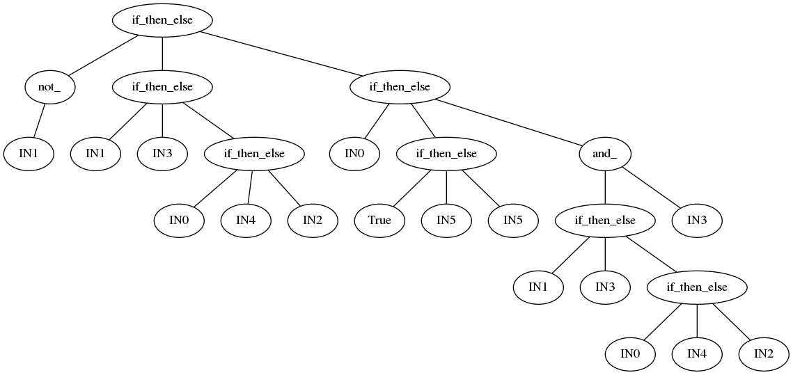
This simple example illustrates how you can actually evolve a simple human-readable solution to the challenge of learning the multiplexer problem. This approach is usually referred as symbolic regression [6]. It also shows you can actually solved with a subset of the operators we provided.
References
[1] https://www.electronics-tutorials.ws/combination/comb_2.html
[2] http://geneticprogramming.com